“Significance is based on sample size and effect size. The larger the sample you have, the smaller effect size you can find to be significant. The larger the effect size present, the smaller sample size you need to find significance. Larger sample sizes are generally better, however any difference, no matter how small, can be found to be significant with a large enough sample size.”
I’ve been talking about how sample size drives the lifecycle of the normal distribution. As the sample size grows the sample size increases and the distribution, which starts out in hyperbolic space where it is certainly not normal.
To simplify our work, we assume normality. We don’t acknowledge that assumption.
rBut effect size matters. The features leading to the effect need to be significant. That effect happens down the tail. The effect happens after you have transitioned down the Makov chain through the states that lead to the effect. Each of those states must be significant.
We need to collect the data from the relevant population before we go there. How agile can we be if we don’t have a population of users to collect data from? How agile can we be if we are not delivering features based on data that is significant?
As I was looking for a distribution that resulted from data encoded as modular data. I can across a prime factorization. I used that factorization to build a distribution that has more than two tails. A normal distribution only shows us two tails. We only deal with two tails.
At the top of the figure, I how a factorization of the system. On the right, I drew a grid that used the values as the height of the tails shown in the original factorization. On the left, I drew a normal distribution that covered the grid. Imagine the red normal as containing the grid. Only two tails appear. The rest are hidden by and within the distribution. The height of the distribution shows us that the distribution is not yet normal. It will get much shorter before it becomes normal. All three figures show the same data.
That was Back in February of 2019, Quanta magazine contained an article, “How a Strange Grid Reveals Hidden Connections Between Simple Numbers.” I read the article. The article speaks in terms of polynomial progressions. I didn’t do anything with it. I went on to slog my way into a thick pdf on generating functions. I could see those functions generating a tail. I could see a statistical dataset as containing a collection of data produced by of one or more generating functions. We usually see that data as being produced by one pseudo-random function. It would be nice if we could get by with one generating non-random function. We are looking for a collection of linear factors from our regression analyses. We could call that a tail.
That was before I took up the regression to the tail phenomena. Regression to the tail happen when an outlier pushes a post-normal distribution, a distribution wider than six standard deviation, to a failure. That happens when multiplication is involved. A post-normal distribution is lower and wider than the standard normal distribution. A post-normal distribution happens as the sample size increases beyond that of a normal distribution, after the normal is achieved.
So this weekend, I came across another Quanta article, “Mathematicians Catch a Pattern by Figuring Out How to Avoid It.” This article from November 2019. This time, the content was nicely tied to the regression to the tail phenomena. So was the data to be sampled from an arithmetic progression or a geometric progression? Is the data added or multiplied from one value to another? Doing the math and filling in those tables tells you which is which. Once you know that you are dealing with a geometric progression, you can put a homological barcode in place. Every data point added to your post-normal distribution might cause a regression to the tail failure. Is that data point an outlier? Is that data point highly leveraged?
The pre-normal distribution has two asymmetric tails: a short tail and a long tail. Only the long tail contracts as the pre–normal distribution approaches the normal distribution. The difference in those tails give rise to a cyclide. The post-normal distribution has two symmetric tails. The similarity in those tails give rise to a torus. A cyclide and a torus are topological constructs. So in wanting to be proactive about regressions to the tail, we can rely on the homological barcode, a tool from topological data analysis, and the barcode’s statistics to inform us as to outlier-driven post-normal failures.
I’ve written abut what to do with black swans, regressions to the mean failures. I am still looking for what to do about regression to the tail failures. What data analysis has to be done? What processes are involved? What organizational structures are essential? What can we ignore? More thought to do. Stand by.
We can see these two articles as being indicators of time. The first article is harder. The second article is easier. That is what we expect from the technology adoption lifecycle. The underlying mathematics got simpler. The underlying mathematics got contextualized in a more useful manner, where it can be turned into a practice useful to people who would never do that mathematics otherwise.
Last night I looked at Rita McGrath’s weekly podcast. This week’s podcast presented “Jumping a new “S” Curve” on July 17, 2020 in McGrath & Whitney Johnson Fireside Chat Full Session.
Johnson worked with Clayton Christensen. She applies his conceptualization of disruption to herself. She wants the individual employee to disrupt to disrupt themselves.
I had to Google Whitney Johnson’s S-curves. The list of hits was short. One of the hits was a link to McKinsey. Foster was a director at McKinsey. Foster wrote the first book on disruption. That book was written back at the dawn of the internet. Foster saw disruption as an accidental side effect. Christensen saw disruption as something that could be done deliberately.
HBJ’s claim that Christensen was first author of disruption was a bit much given that Christenen cites Foster in Inventor’s Dilemma. Christensen eventually claimed that no S-curve was necessary. Wikipedia published that claim at some point in the past. I was interested in discontinuous innovation long before Foster. Various disruption pushing professors surrounding Christensen have tended to replace discontinuous innovation with disruption, but disruption is not about invention, or S-curves, no discontinuities. In fact, Christensen’s disruption is about a point in the technology adoption lifecycle that is continuous in regards to the carried content.
As a result disruptive innovation has come to replace discontinuous innovation. One thing got lost, the technology adoption lifecycle. One disruptor captured a billion dollars in investor money by claiming disruption. This long before it actually disrupted anything. The VCs are funding predatory pricing in the hopes of capturing a monopoly position. Still, the end of the technology adoption lifecycle is closing the window on the category. The category will die before the justice department gets involved.
Disruption is about the business model. Disruption is not about invention, or the innovation.
Another discussion on the Fireside Chat this morning is how managers want to be designers. Design thinking is all the rage. B-schools created design thinking. Yes, some continuous innovation. Enjoy, be happy. The category is dying. We exit that business before disruption happens to us. Facing disruption, we must innovate discontinuously in an ongoing manner.
These two Fireside Chat discussions leave us with managers that to innovate without inventors or designers. Oh, well.
“Of magnitude that which (extends) one way is a line, that which (extends) two ways is a plane, and that which (extends) three ways a body. And there is no magnitude besides these because the dimensions are all that there are.”
“The Journey to Define Dimension,” Quanta Magazine, September 13, 2021.
So what would that mean to product managers?
“Yet, as we shall see, mathematicians discovered that dimension is more complex than these simplistic descriptions imply.”
Spaces insist on their own logic and arithmetic. In statistics, the dataset insists on its own space.
Every continuous innovation extends the existing theory, the known theory, the theory that informs us as to how we do what we do in that existing dimension. Continuous innovation extends the current dimension. A discontinuous innovation, however, births its own theory. That birthed theory is independent of other theories. It gives rise to its own independent collection of new dimensions, its own ontology, its own meaning, its own epistemic culture, and its own samples. It gives rise to an independent dataset.
Samples give rise to that discontinuous innovation. The inventor captures the relevant distribution before the marketer. The inventor has a network of other inventors working in domains relevant to that discontinuous innovation. The inventor has a bibliographer. The inventor participates in their invisible college. The inventor reports their work in journals, and solicits citations from other researchers. This happens long before workers incorporate that discontinuous innovation into their work, and long before managers get involved.
A workers we go to school to get a job. We are taught known theories. We take classes that enable us to work at professions at the leading edge of our professional domains. We learn our way in. We also learn our way into our into our hoped for professions. We accumulate and commit to contemporary theories. We get exposed to some new theories.
We might get hired to implement those newer theories, each a new theory from a discontinuous innovation. The people hiring us were educated in a prior, older theory. They might not know how to adopt that discontinuous innovation. They might not know what that discontinuous innovation means in terms of the work done in the workplace. They might not know how the work is done, the practices around that work, or how the workers will come to define their profession, and their own professions. The adopters will learn these things in some eventuality. They don’t know yet. Neither do you. But, if they hired you to bring that discontinuous innovation on board, it will be because you are have more familiarity with it than they do. Act like it. You are the expert.
But, that expertise has its limits.
It the technology is coming in from the IT department, it might have skipped the functional unit doing the actual work. IT people know the carrier. They don’t necessarily know the carried content. Desktop publishing was adopted by publishers that understood the carrier, but Steve Jobs became a hero because he understood the carried content, which raised the expectations of the underlying software. Software is media. Newspapers are a media. The news we watch on TV is more obviously a media. But those media don’t tell a story the same way, or to the same ends. Newspapers in WII thought us into a war. Television had us watching and arguing our way into a very different war. Different carriers in the software as media model facilitate the same carried content to different different ends.
Software a media divides the expertise. Software can be used without knowledge of the carried content. Some employer want tool users. Knowing those tools doesn’t mean that the carried content is known.
The software as media model in embedded in the technology adoption lifecycle (TALC). The focus on carrier and carried content oscillates in importance over the lifecycle of the innovation. The software as media model plays an essential role in the B2B early adopter engagements. The first sale is to an early adopter. Their business is built delivering the work product of a functional unit. The focus is on the work, not the technology that enables the work, and work is the carried content. The carrier is built up to from that early adopter.
The TALC phases are ordered. It is not random. The TALC is organized by the level of task sublimation that its application presents. That level of task sublimation serves and attracts a specific population of users. While UXers are taught to deliver simplicity, the TALC initially delivers the complex. Many releases later, as the TALC moves into later phases, the application achieves simplicity. One TALC phase leads to the next phase. Skipping to a specific phase can be done, just understand, that doing so will cost you time and money. Randomizing the ordered processes randomizes the user populations and the readiness of the learners. Focus on the business processes and the organizational structures that own each of those processes.
The vender organization begins their market development efforts for a technology birthed with a discontinuous innovation to an early adopter brings the technological enabler to the work. The early adopter has the product visualization. The early adopter has also has the value proposition. The early adopter have thought about that value proposition for a long time. That early adopter are the gateway to their vertical market. They have a network in that vertical market. They know people. They lead people. The people in the vertical market know the early adopter, and expect that early adopter to lead them. Those people in that vertical market will watch the success of that early adopter’s success to ensure their own success. It is unlikely that the early adopter’s vertical market is served by a trade journal. It is unlikely that you as the vendor can buy your way in. Personal selling works. Trade journals less so. “We did not crossing the chasm” is what seral entrepreneurs say when they exit. They tried to buy their way in, rather than doing the harder work involved in personal selling.
So what about dimension? Well, regression requires us to focus on one dimension. It crosses another dimension at some angle. That angle tell you about the relationship between those dimensions. If a relationship exists, we can move off our familiar direction and head in the direction along that new dimension. We can traverse one step at a time along the Markov chain explored by the regression analysis. With each step, we have another regression analysis to do.
Serve the vertical market well. Ensure the success of your first B2B early adopter.
I’ve been looking at requirements engineering lately. Requirements engineering has a lifecycle just like the technology adoption lifecycle. That is convenient because it gives us multiple tails, which in turn lets us leverage simultaneous development of the epistemic change. It gives us numerous topics to learn and a way to staff the effort so we can be ready to capture the lessons taught by the early adopter’s organization in our bowling alley.
When we learn statistics, we learn that there are two tails. We see this in our 2-dimensional figures of the normal distribution. Those figures compress an n-dimensional distribution down to two dimensions. Those figures hide n-2 dimensions from our visualization. We only see two tails. But, in a YouTube tutorial on linear regression, we were replacing the linear functions from a prior regression analysis with new functions. Why?
The lesson was designed to teach us something. That something was something we probably not something we needed to learn. It was just another demonstration of where we end up when we throw away outliers. We end up confusing tails as well.
Keeping those tails distinct is something we can achieve in our tails. Our software applications present a user with a chain of user interface controls. Those chains can be seen as Markov chains. Each control or user interface element translates into a state in at least one Markov chain. Each control or element has a use frequency. Those use frequencies order the chain into a tail from the highest frequency to the lowest. Think of each control as a can of soup that has a UPC code printed on it. Each use adds another can of soup to our basket that we put through the cash register.
When we build our software, we order our controls. That, in turn, orders our tails. There are numerous controls that give rise to numerous tails. There are no surprise tails. There are no surprise outliers. We won’t be wondering about factors unless we are dealing with a bug. That bug would alter the frequencies in its relevant tail.
You are starting to see that product managers must teach the application to the developers. Marketing teaches the users. Users teach the developers. It sounds like a mess but discontinuous innovation, innovation that starts with a new theory, a new ontology seeding a new collection of dimensions, simplifies and aligns the teaching and learning. The customers, users, clerks, and managers have much to learn. They are doing something new. The old practices only worked once the prior, now current, theory was put into practice. We are putting the new theory into practice. We must learn those practices. Our software will implement the automation now possible around those emerging practices. Much will change.
A discontinuous innovation delivers economic wealth because it is different, emergent, and justifiable. It delivers a different constraint envelope within which the new practices get done. The application constructs an emergent culture around itself. That culture directs the future direction of the application, the prospects and future customers, and future practices. Nothing is static yet. Being a commodity is years away, profitable years.
Right now, the application embodying that new theory is for experts. Those experts work for the B2B early adopter in a vertical organization. They don’t need task sublimation yet. The practices are emergent.
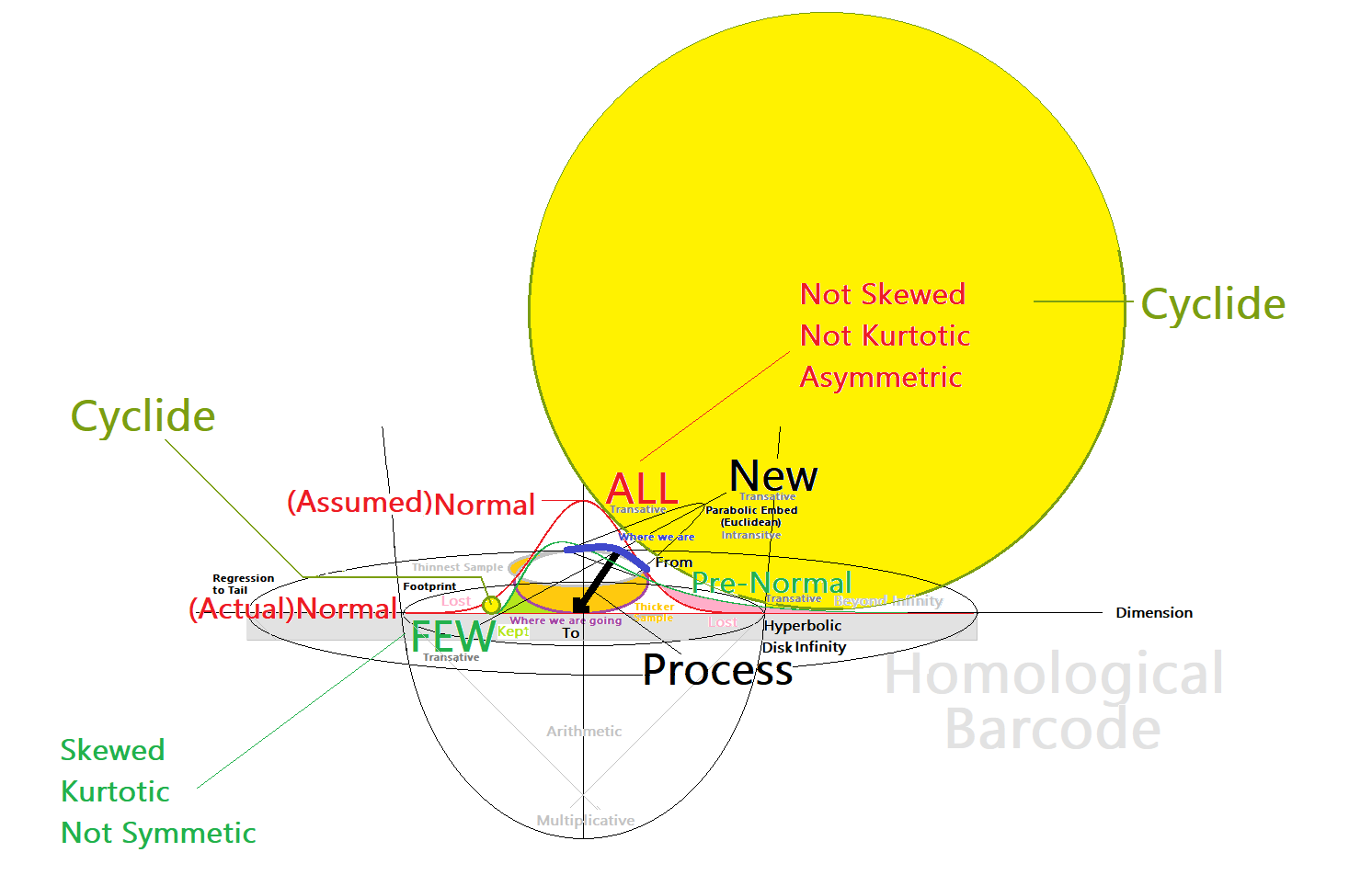
I drew a figure this morning. I could not find the figure that that contrasted the Gaussian and Lebesgue probabilities that jointly give rise to the unit square view of the sample space where Markov Chain integration gives us a probability density that in turn allows us to define the geometric spaces in the sample space. I will keep looking for that figure. Anyway, this morning’s figure tied some new ideas together.
I started this figure with a red, single-colored standard normal, N(0,1), where the mean is 0, and the standard deviation is 1.0. When we start to sample, we have not yet achieved a normal. I call this a pre-normal. It is shown in green. As we collect more data we achieve the normal. But, we don’t ask ourselves is it normal yet. We assume normality. But, eventually, we achieve normality, aka actual normal. The actual normal is shown in red.
With a radius of three standard deviations, the normal will exhibit a negative event as an aggregate of three events in a Markov chain presented to the normal as outliers. Those three events drive a black swan event in the standard normal. Those three events exhibit regression to the mean.
With a radius of more than three standard deviations, the normal will exhibit a negative event with less than three events in a Markov chain or with one such negative event. These much shorter Markov chains exhibit a regression to the tail.
I revolve a torus around the standard normal. If it was shown, its torus would lay on top of the red normal. It would appear as two circles of the same size on each side of the normal. That torus would exhibit symmetry. That torus would not be orientable.
What I’ve shown is that the pre-normal has a cyclide surrounding the pre-normal. The yellow cyclide of two parts appears as a large yellow, maximal-sized circle and a very small, yellow, minimal-sized circle. The shape would exhibit both eccentricity and curvature that would ensure the topological object was snug with its pre-normal. That pre-normal distribution is asymmetric. The cyclide’s minimal and maximal-sized circles of the pre-normal orients the cyclide. The cyclide is asymmetric a well.
The white area between the yellow sphere and the green distribution is an error. Because of the eccentricity and curvature, I cannot draw the pre-normal and its cyclide as being snug. In an accurate diagram, the normal distribution and the cyclide should be snug.
The minimal circle represents the short tail of the pre-normal distribution. The maximal circle represents the long tail. , The maximal circle shrinks to the minimal circle as it rotates towards the minimal circle. As the cyclide continues to rotate through the minimal circle, through the short tail, the minimal circle grows as it rotates towards the maximal circle.
The normal distribution exhibits a sequence of changes as the sample size increases. The figure calls out the properties of the pre-normal distribution as exhibiting skewness, kurtosis, and asymmetry. The figure also calls out the properties of the normal distribution as exhibiting no skewness, no kurtosis, and symmetry.
Within three standard deviations the normal exhibits regression to the mean. The first ellipse out from the mean shows us where the three standard deviations of the standard normal ends. In the hyperbolic space that the pre-normal finds itself, that line ending the standard normal can also be seen as the near infinity of that hyperbolic space.
Beyond three standard deviations, the normal exhibits regression to the tail, the long tail. The Markov chains shrink as we evolve to a regression to the tail situation. The figure shows a homological barcode under the x-axis when the distribution reaches beyond the three standard deviations of the standard normal, or when the distribution exhibits regression to the tail.
The distribution near the short tail is stable, shown in green. The distribution near the long tail is fleeting, shown in pink. Investments near the short tail will persist. Investments near the long tail will vanish.
Entrepreneurial undertakings should focus on the question of serving a few customers or serving all customers. We can do the former with smaller samples, so we can do it quicker. We can do the latter with larger samples, so it will take longer to get it done. So the decision focuses on the few and the all. The “few” can happen in the pre-normal. The “all” can happen in the normal or more typically post-normal, but not in the pre-normal. The “all” happens in the normal. In TALC terms, “all” happens in the late mainstreet phase. “All” happens once you have achieved commodity status.
I started this figure thinking I would move from an upmarket position, the thick blue line, and move into a downmarket position via processes that appear as a thick black line. Price changes can trigger these market segmentation moves, but there is much ethnography needed. The orange area shows the area that needs sampling. That sampling takes time.
I’ve attended to the differential normals. I do that to deal with non-Euclidean spaces. On the figure, I also wanted to deal with parabolic space. I divided the thick blue line with a line that serves as the axis of a parabola. The parabolic space is embedded. It exists in Euclidean space regardless of sample size.
A homological barcode has its own statistics independent statistics, a statistics of the distribution. The outliers are multiplicative. Multiplicative processes are the drivers of regression to the tail situations.
So what do we make the diagram’s word salad? We sample. As we do so, we birth and raise a normal distribution. That distribution can undergo a black swan. That distribution can eventually become a post-normal distribution, a platykurtic distribution, a shorter and wider normal, a normal where the standard distribution is wider than 1.0. The post-normal distribution is born as pre-normal distribution, a platykurtic distribution, a taller and skinnier distribution.
The pre-normal and normal distribution exhibits regression to the mean. The post-normal distribution exhibit regression to the tail, the long tail, the tail that vanishes when multiplications cause outliers whose distances from the mean are too far from the mean, outliers that are highly leveraged.
We throw away outliers. We ignore them. We lose them in our interquartile ranges. We don’t ask about the length of their Markov chains. We don’t bother making the regression to the mean or the regression to the tail questions. We let the consequence happen because risk happens. Never mind that we put homological barcodes there to prevent the expression of those risks, and to live longer than those risks.
We can detect the regression to the tail event. How are we going to react to them? What architecture do we want to be in when we react? The black swan events let us with these same needs. I’ve demonstrated that we can be proactive about the black swan events, about events exhibiting regressions to the mean. Similarly, we can be proactive about events exhibiting regressions to the tail.
A few months ago, I was walking down a street that was familiar to me. But, many of the businesses on that street were new to me. I’ve not been inside. I haven’t seen what they sell. I haven’t experienced the place. I have no idea as to whether I would ever enter those places. They were the “New.” That’s B2C. That walk was a matter of walking under a series of normal distributions. That walk is a sampling process. If it is familiar to me, its a normal distribution that has achieved normality. That normal is in Euclidean space. If it is unfamiliar to me, it has not achieved normality yet. It sample size is too small. I’ve called these normals the pre-normal. The pre-normal is in hyperbolic space. It needs more sample data before it achieves normality, or Euclidean space. The unfamiliar areas that we traverse have a logic and arithmetic that differs from the logic and arithmetic of the familiar areas we traverse. This latter space is the ambient space, the Euclidean space. The post-normal, other much more familiar areas we traverse, the post-Euclidean space differs from the space of both the pre-normal and normal in regards to its logic and arithmetic.
Change in sample size changes the geometry of the normal distribution. The normal distribution exhibits a lifecycle.
The technology adoption lifecycle (TALC) change as well over the life of the technology it describes. I do discontinuous innovation, so I’ve been focused on the distinction between continuous vs discontinuous innovation. It has economic outcomes. Economic wealth accumulates via discontinuous innovation. Continuous innovation accumulates cash without regard to economic wealth. Understanding the difference is important, but the difference has been mostly lost. We learned the wrong lessons from the dot bust.
Discontinuous innovation is not more risky. It happens before a mass market exits. It happens in hyperbolic space while we ignore that space and insist on doing our analysis in Euclidean space. There is a process. But, we ignore that. We insist on the business orthodoxy, an orthodoxy that works exclusively for existing mass markets. Those existing mass markets have large samples which give us post-normal distributions. These port-normal distributions have a geometry that exhibit a linear, Euclidean geometry.
The pushers of governmental subsidies for innovation programs base their anticipated results on discontinuous innovations but only end up funding programs built to create or replicate continuous innovations. It sounds “New.” They sound like extensions of the past, like an extension of the old theory. These programs work, but only for continuous innovations.
I’ve followed the TALC and put the discontinuous innovation phase in front of, earlier to, or prior to the continuous innovation phase. The TALC consists of six, or seven phases. Those phases have their own unique business processes. Each of those phases has its own organizational unit. Each of those organizational units runs itself for its own purposes. Each of those phases serves very different users. The orthodoxy delivers only one of the phases, the late mainstreet phase. They don’t need VC monies. They should be getting a loan from their business banker.
In , my readings around the TALC, I read a paper from a researcher that looked for an attractor basin that could be used to predict a technology vendor’s phase on the technology adoption lifecycle. Apparently, that the TALC s organized around the level of task sublimation required to serve the prospects in a given TALC phase, was not known to that researcher. But, the researcher used trailing indicators. The researcher found what he sought. Why would a vendor rely on trailing indicators? That vendor should use their internal processes to tell them exactly from what TALC phase in which they find themselves. But that depends on their process management.
Startups evolve. Innovations evolve. Vendors evolve. Users evolve. Use evolves. It starts to sound like software evolves. It sounds like software engineering and architectural, or organization structures as enablers. Yes, data structures.
So I’ve put discontinuous innovation and continuous innovation in their own divisions. Those divisions manage their phase-specific companies. The bowling alley takes a new theory to an early adopter. That early adopter runs a very specific functional unit in a vertical market. Once the vendor develops six functional unit, or six vertical-market applications, or applications for six different early adopter applications, the vendor can aggregate those six applications, applications built on the same new theory, aka the same technology. The vendor widens the IT integration of those applications. Then, the application is ready to enter the IT horizontal, aka is ready to enter the tornado.
We can draw the organizational structure as diagrams, as I have been. But, you have to hire. Then, you have to train the hires to run their business to the prospects of the TALC phase they serve. Each of those businesses gets its own business rules in the vendor’s database. Those business rules embody and enforce those diagrams. This advice about the use of business rules is key. These partitions are everywhere. That person you hired to do the usual job in an unusual, aka “New” circumstance, is inside one.
Another element is how the surveys evolve over time. That survey data runs from zero to infinity, but we use datasets and assert normal distributions to avoid dealing with this migration across spaces and their logcs and arithmetics. The distribution migrates from hyperbolic space to Euclidean space to spherical space. Statistics emerged back when math was still insisting on being Euclidean. Each of those spaces determines the logic and arithmetic in that space.
We apply machine learning without reminding ourselves that machine learning insists on Euclidean space. But, we call out this a failure of machine learning. Researchers are trying to convert data from hyperbolic spaces to Euclidean data, so machine learning could work in hyperbolic space natively. Native machine learning is still failing. It will continue to fail until we attend to the differential nature of our distributions. When different entities have their own business rules, the proliferation spreads out the spaces where ambient machine learning fails.
The advice of late goes further than Iever have. Every “new” should be embodied in its own business rules. When I was hired to bring the concept of product to an established company. I came from a product company, but the company that hired me was not a product company. The hiring company never became a product company. The proposed new company never ran itself according to its own organizational structure, nor to its own business rules. My bad. I was the “New.” My opportunity. In the longer view, I see those business rules everywhere even in the absence of business rule boundaries. The old organization resists change. There is much it does not know about itself.
Woke up this morning thinking about persistent homologies after a long night watching topological data analysis videos. I didn’t take notes on that content until a few things were screaming at me. I was watching David Damiano’s Applied Topology – 2020, a twelve-part series from YouTube’s Applied Algebraic Topology Network. I’m nowhere near finished with that series of videos. Learn some linear algebra before diving into computational topology.
The content screamed when it defined outliers as aberrant data. In statistics, we arbitrarily throw out outliers. We’d rather be blind. We use datasets rather than data. We use compressions of distributions, so we end up with binomial or multinomial distributions. We do the latter because we can only see three dimensions, and we compress those dimensions into two dimensions most of the time. We know that we are doing multidimensional statistics. There are more than two tails in our data, but we can only make statistical inferences with two distributions. Multiple nomials mean that we have not separated the dimensions in the data. Not insisting on seeing the long tail and the short tail pair of every dimension screams loudly that we are gambling, rather than investing. And, we insist on Euclidean spaces. We insist on normals and orthodoxy when all things new have sample sizes that are not normal yet. Neurons in our neural networks insist on Euclidean spaces as well. Yeah, screaming. No wonder machine learning requires so many examples before it learns.
No more screaming.
In yesterday’s blog post, I proposed using the length of the persistent homology as the basis for the distributions that exhibit regression to the tail. Finding the mean and the standard deviation in those distributions is an intractable problem. Finding the length of the persistent homology is not intractable. Those persistent homologies, aka barcodes, are interrupted by outliers. Start with a tessellation of triangles. Find the adjacent triangles. Those pairs give you a cycle. Once paired that cycle births a dimension. And, when the persistence ends, the dimension dies.
From a product strategist’s perspective, the point of discontinuous innovation is to birth categories. The technology adoption lifecycle (TALC) is a graphical representation of the life of a category. A category is born. Eventually, that category dies. MBAs spend most of their effort extending the life of their products, companies, and industries all of which reflect the life and death of their category. Economic wealth is generated by new categories. Cash is involved along the way, but cash s not economic wealth. Cash is an investor’s mismeasure of innovation. Cash is not the point. These days someone out on LinkedIn said, “we cut wages to compete,” thoughtlessly.
Our continuous innovations keep the category alive. Innovate or die. Well, not so fast. But, I’ll let those myths alone for now. The business orthodoxy can’t handle it.
Anyway, these lifecycles show up in theories, ontologies, constraint envelops, features, products, samples, use as samples, curriculum marketing as samples, differential distributions, and persistent homologies. But when did you last remove a dimension from your buisness rules? Does every “new” in your companies have its own organizational unit iwht its own business rules? Or, did your last “new” fail, because you ran it just like you run your existential organizational units. Did your company’s immune system fight your last “new?” Are your VCs allowing you to birth a category? Have you organized your company to maxmze its ability to quickly learn from its “new”s? Do your barcodes get addressed by your businesss processes? In your SOX doumenation? Are you ready and able to teach the “new?”
Do you make decisions only in an ambient, Euclidean space? Can your company operate natively in hyperbolic and spherical geometries without encoding and decoding the data traffic to and from those spaces? Warning machine learning continues to assert Euclidean space. No wonder data scientists find that does work in so many situations. Even your business banker asserts and insists on the spherical geometries. Your last startup might have failed because you and your associates insisted on running your hyperbolic, aka “new,” business as if it were spherical. Blame? Not crossing the chasm? The frying pan was wrong? No, the maths and the logics were wrong! And, of course, you bought ads with the money your VC gave you, instead of mapping out your B2B early adopters first three degree of separation and did personal selling to that network. Of course, your industry might have saved you by not having a trade magazine, which means you couldn’t buy your way in.
Back to the math.
One more scream. I looked at some content on data visualiation this morning. It is too wrong. There are nine modals. Yes, I count past nine. That means hthat there are nine different normals compressed into one distribution. Actually, there is a thick tail that falsely counted as a normal. What a mess. Why is this a problem? Topological data analysis expets to see one normal on top of the next, normals all the way down. This in layers. Subset within subset within subset within … Every one of those subsets have their own barcode. Those layers of normals is what they call a filtration.
The histogram bars must mut be under the distribution, or again, not a filtration.
Back to barcodes, a geometry.
I’ve talked about the difference betweeen circles and ellipses in coreleations. In regression, perpendicularity, or orthogonality, means there is no correlation between the intersecting dimensions.
In the figure, the thick black lines, aka the barcodes, intersect. The interections are open (unfilled) or closed (filled) points outlined in red. The open point of intersection has no correlation so it appears as a circle. The other intersections are closed points. These closed points should be shown as ellipses. Correlated intersections show up as ellipses. The barcodes show a triangle in Euclidean space. In hyperbolic space, a triangle has less than 360 degrees, shown in blue. In spherical space, a triangle has more than 360 degrees, shown in orange.
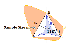
A normal begins with the assertion of a random variable. When asserted, the random variable shows up as a line to infinity. It is a point. There is no interval, so there is no probability. So we take a collection of samples, which spreads out the probability mass along a dimensional axis. A histogram results. That histogram is peaked, aka very tall. As the histogram gets wider, or the barcode gets shorter, the histogram become less tall and wider. That tall distribution is pre-normal. That shorter, wider distribution achieves normalality. It is only normal for a short period of time at some sample size of n. The distribution becomes even shorter, and even wider as the sample size exceeds the number of sample points needd to achieve normality. These distributions are post-normal. That is the lifecycle of the normal distribution, from birth to death.
This diffential view of the normal appears from the assertion of the existence of the underlying random variable, the dimension. I’ve shown the initial, singular histogram bar as the mean. I’ve drawn a time axis away from that mean. Hyperbolic triangle (H) appears in blue. It bulges inward from the the black Euclidean triangle (E). The orange spherical triangle (S) bulges outward from the Euclidean triangle. As the sample size m gets larger the distribution grows outward on the figure. Normals squat, aka get shorter, and its standard deviation gets wider.
In regression to the tail situations, the Markov chains involved become shorter. The distribution becomes increasingly fragile. In regression to the mean situations, the Markov chain involves a network of three or more nodes, which means it takes three or more events to trigger risk expression. The regression to the mean situations happen in hyperbolic and Euclidean spaces, at aka pre-normal and normal sample sizes. Both of these regressions happen on the long tail side of the distribution. Seeing the skewed distribution, rather than the asserted normal distribution is key.
Regressions to the mean happen in situations built with addative opertions. Regressions to the tail happen in situations expressed in multiplictive operations. The usual discussion of the latter mention lognormal distributions. Know the math of your processes. Make the math of your processes in your BPM system. Beware of multiplication. One problem is how we preplace multiplication with repeated addition. Logs replace multiplicatins with additions, so we can hide regressions to the tail, which helps us hide the statistical realities and our obliviousness.
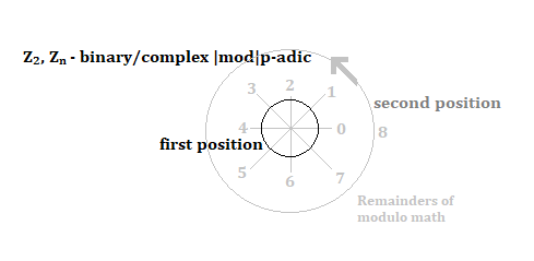
Keep in mind that exponential situations do not got to infinity under some game theoretic rules about not exceeding the value of the game. When the value of the game is exceeded, the underlying situation becomes negative. As an example antitrust enforement kicks in. The math of p-adic polynomials act as a break on exponentials, because p-adics expresss multiplication like complex numbres as rotations around the unit circle.
What is growth under this latter mathematics? Growth can be expresed in TALC terms. An addressible market is a discreet thing. Your product will traverse phases of the TALC without growing. Grow to consume your market faster. But, that exposes your company to ethnographic changes well beyond price.
So lets look at the TALC as the sum of n N(0,1) distributions. Here n would be 7 if you included product-led growth (PLG) as a phase where you sell and serve cloud-based, horizontal applications. The internet 1.0 bust removed the precursor phases to the tornado. from the TALC, so the entry to the tornado is now called the chasm. The chasm used to be at the entry to the vertical that led to a market leadership position in the B2B early adopter’s (clients) vertical markets. Those markets did not have trade publications pushing marketers to put their marketing dollars into personal selling and network marketing efforts. The TALC still matters.
Disruption is about category death. This language hides the absense of discontinuous innovation, jobs, economic wealth, and the fact that venture capital is now being used to buy monoply positions via preditory pricing. Nonsense really given how near category death is.
One particular VP of sales that we had would always close his discussions with “Back to work!”
Topological data analysis generates barcodes as a means to determine the length of persistent homologies found in sample data. I’ve drawn tori and cyclides over normal distributions in several earlier posts. The tori happen when the distribution is normal. The cyclides happen when the distribution is pre-normal. Sample size drives the distribution from hyperbolic space to Euclidean space, and from Euclidean space to spherical space. The distribution is differential. I have yet to find that to be the case in topological data analysis. I don’t find that statistical distributions are differential either. But, I have found that in a recent study of Covid patients where machine learning was applied to determine treatment outcomes of individual patients, the geometries of the spaces were in conflict. The samples were prenormal, or happening in hyperboic space while machine learning happens in Euclidean space. Doing machine learning in hyperbolic spaces is a contemporary research topic. We assert normality long before normality is actually achieved. We don’t pay attention to how sample size drives the properties of the sample spaces. That tradition of considering distributions to be static and non-differential continues in topological data analysis.
I’ve been looking at convergence to tail situations. Much of the discussion is about knowing the mean and the standard deviation, both of which are unknowable in the distributions having the convergence to tail problem. So in this morning’s research, I found that outliers alter the topological barcodes or persistent homology of the distribution.
I’ve mentioned how a subset of a normal distribution might have a sample size too small to remain normal. These subsets happen in hyperbolic space.
I did find Persistent homology of Gaussian fields in Euclidean space this morning. That article mentioned this article, Understanding Persistent Homology and PLEX Using a Networking Dataset. The latter study used subsets as the basis for a collection of tori each having their own persistent homology, a length. Outliers impact the length of the persistent homology. The outliers impact the regression to tail situations. Perhaps we should look at the homology rather than a mean and a standard deviation that we cannot compute.
The study sought out subsets of brain function data to find evidence of various brain pathologies.The brain is seen as a manifold, so an atlas is used to map brain function data to collections of dimensions. Those dimensions have their own normal. Each of those normals appear in the diagram as a tail. Each of those tails drive the shape of the torus related to each of those tails. Each of those normals represent a subset of the sample data. Those subsets are defined by the atlases describing the brain’s manifold.
The thinking of a corporation could be represented by a cognitive manifold.
One interesting aspect of the subset as torus view is that the length of the persistent homology tells us the radius of the tori. In earlier discussions, I found that a skewed distribution has a short tail and long tail pair. That pair of tails is expressed by a cyclide where the smaller diameter of the short tail increases to the larger diameter of the long tail as the diameter rotates around the normal. This is what makes the pre-normal generate a cyclide, rather than a torus. Rotating away from the long tail shrinks the diameter. This orients the dimension without the need for a correlation.
Looking at the persistent homology’s length provides us with a better way to see the impact of outliers. The orientation of the cyclide provides us with a way to se the orientation of the underlying dimension in a pre-normal space.
Here I am just showing a slice through the three doughnuts or tori generated by the three subset samples. The curvature and eccentricity of the distributions generate the fitness of the tori and the normal.